Today let’s look at how you can get a random row from Google Sheets with Zapier.
There are so many ways you can use this.
- Selecting a random blog post to share on social media
- Promoting a different offer each week
- Sending yourself a random motivational quote each morning
Those are just a few examples but in this video you’ll learn how to actually get the random row.
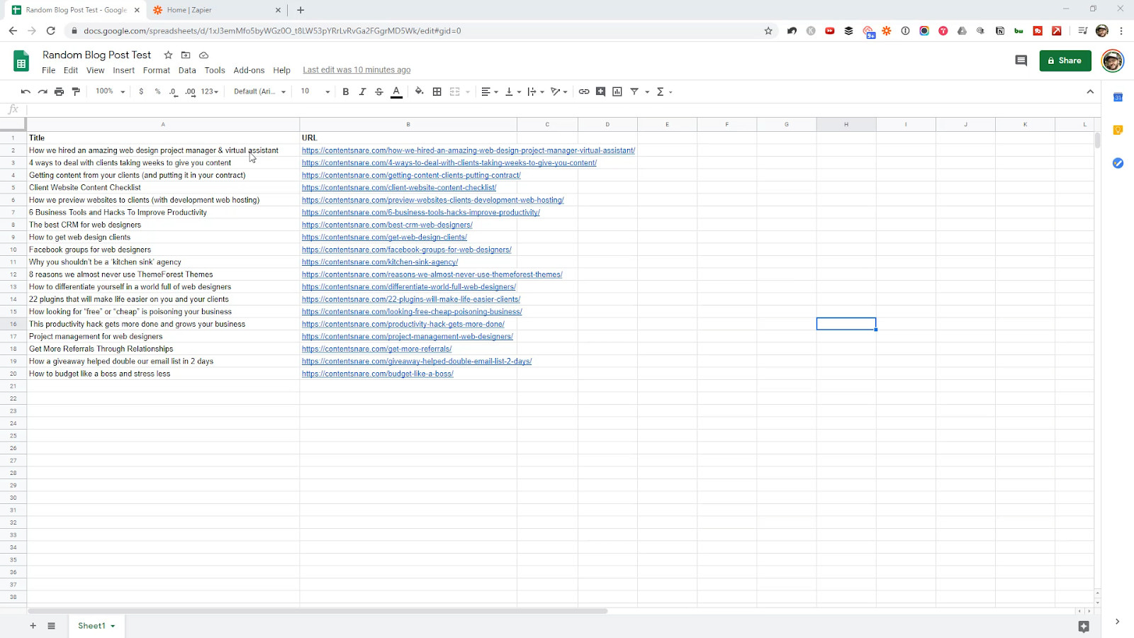
Here’s a spreadsheet of a few of our blog posts. We’ll try to pick a random one of these to share.
Over at Zapier, let’s create a new Zap.
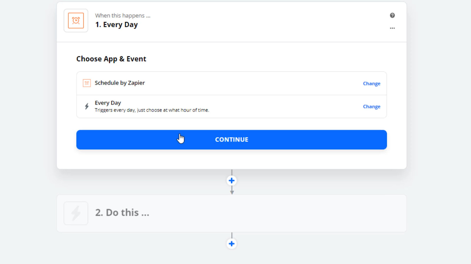
We need to decide on a trigger, and to keep this simple let’s run this Zap at 9am every day using Schedule by Zapier.
The next step is to look up a random row in the sheet. But to do this we actually need 3 steps. We need to
- Find out how many rows there are
- Generate a random number
- Get the row that matches the random number
Set up the spreadsheet
We’ll need two new columns in the spreadsheet.
Row Number
This will be used to pick the row once we’ve generated a random number. Just use the formula
=ROW()
Has Value
This will be used to find the last row that has something in it.
=if(ISBLANK(B2),””,TRUE)
Every time you create a new row, you have to make sure that both of these formulas are filled down into the new row. Sometimes Google is smart enough to automatically populate new rows with the formula.
But there is a trick to make it always work. It’s a little bit advanced. First, delete everything from those two new columns and put these formulas into row 2.

Row Number
=ARRAYFORMULA(if(ISBLANK(B2:B),””,ROW(B2:B)))
Has Value
=ArrayFormula(if(ISBLANK(B2:B),””,TRUE))
ArrayFormula automatically populates every row with the same formula. There is some checking in here to make sure that we only add values to the row if the URL is not blank.
Get the last row number
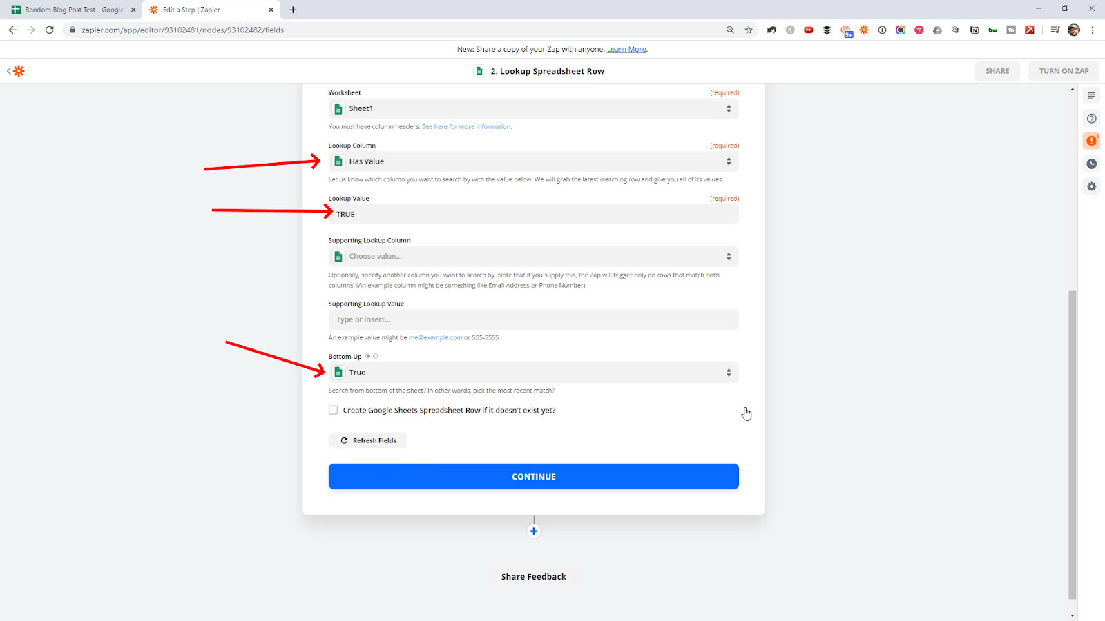
Back over at Zapier, let’s get the number of the last row.
To do that, we’re going to find the value TRUE in the Has Value column, using a Bottom-Up search.
Generate a random row number
Now we need to choose a number between 2 – because that’s the first row with a blog post in it, and the last row.
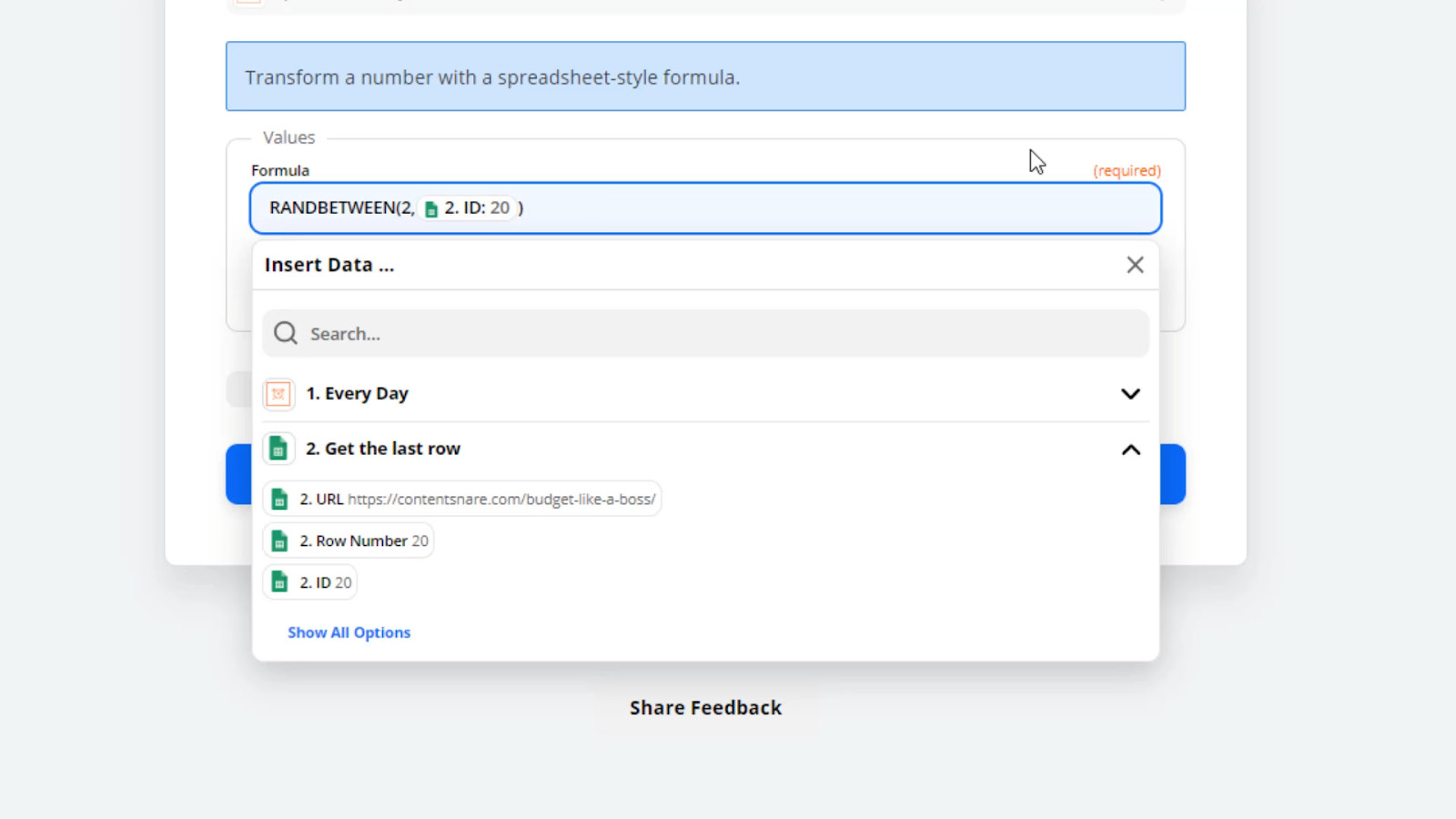
For that, we’ll use Formatter by Zapier – Number – Spreadsheet Style Formula and enter this formula
RANDBETWEEN(2, {Last Row Number}) like you see in the screenshot below.
Choose the row based on the random number
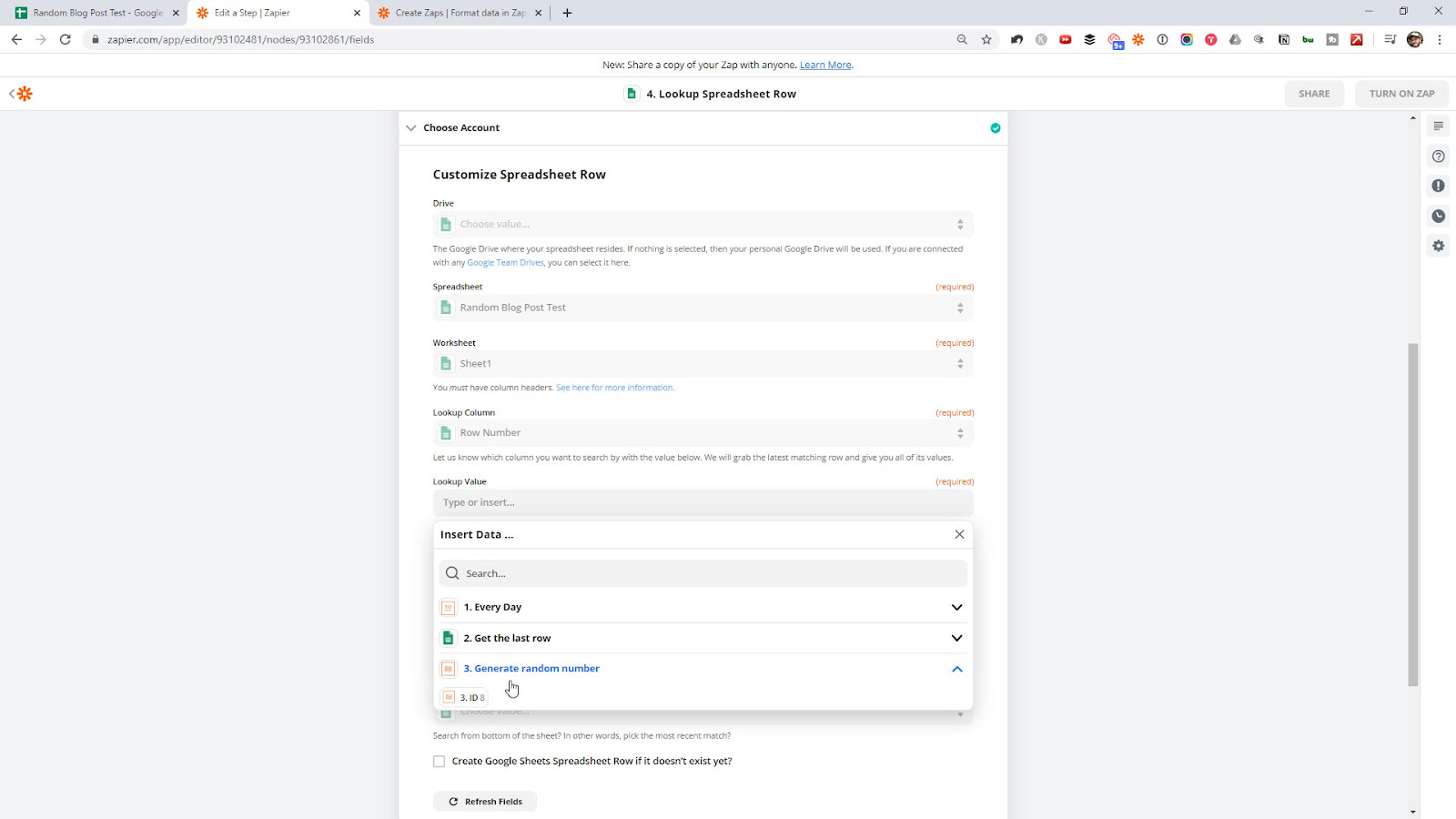
Finally we use a Lookup Spreadsheet Row action to find a row based on the Row Number column that was created earlier.
Share the blog post
Now the next action depends on what you’re trying to do. If you were sharing a motivational quote with yourself, you might email it, or add it to a slack channel for all your team to see.
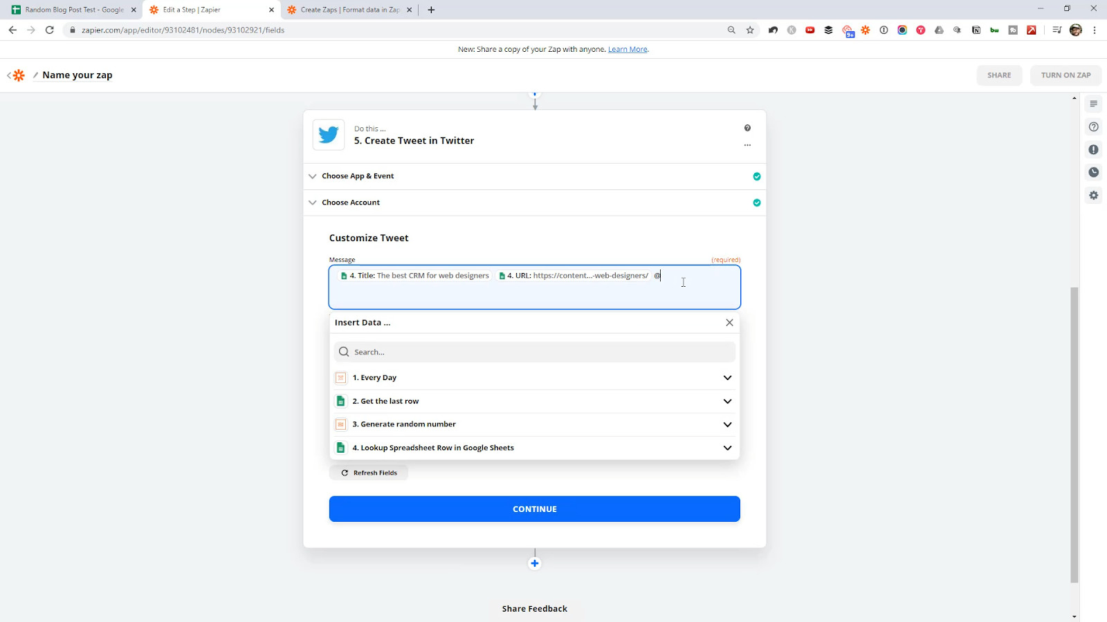
In this case, we’re going to share the blog post to Twitter.
That’s it!
You can use this same method to get a random row from any kind of spreadsheet to use in any of your workflows.